Pico is a programming system that is constantly in a so-called Read-Eval-Print-Loop or REPL. Upon entering an expression, Pico will check the syntax of the expression (i.e. read), will evaluate the expression in order to yield a value (i.e. eval), will print the result on the screen (i.e. print) and will subsequently be waiting for a new expression to be entered. The following short tutorial explains the basic kinds of expressions that Pico will accept and discusses the kinds of values it prints when evaluating these expressions.
Content:
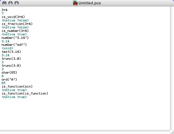
Pico knows seven kinds of values: numbers (i.e. integers), fractions (i.e. reals), texts (i.e. strings), symbols (i.e. quoted identifiers), functions, tables (i.e. arrays) and finally, void, the empty value (later on we will see Pico also features continuation values and dictionary values, but it's too early to introduce them already). The following transcript shows how the basic values can be used in an interaction with the Pico REPL:
Pico is a dynamically typed language. This means that variables do not have a type. Variables just contain values. On the other hand, every value does have a type. Pico values can belong to one of the seven Pico types :
As said, Pico variables have no type, so it is possible to assign a value of a different type to a variable than the type of the value it already contains. Of course you have to make sure that no run time errors will occur, when that variable is used within an expression. The following native identity fuctions can be used to find out the type a certain variable has at a particular time. It is applied to any Pico value. The result is either true or false (notice that there are no booleans in Pico. true and false are functions - more about this later):
Pico also has 6 type conversion functions to switch back and forth between different types
The following screen shot exemplifies these concepts in an interaction with the REPL:
The Pico REPL works with respect to a dictionary, a collection of variables "currently" known by Pico. The dictionary has to be though of as a linked list. Definition new variables adds them to the end of the list. Looking up variables starts at the end of the list and proceeds upward to the beginning of the list. At Pico system startup there is a "global dictionary" already initialized to contain a number of primitive names, associated to built-in functions.
There are three things one can do with a variable: define it, assign it and refer to it. Reference is done by simply evaluating the variable. Definition happens with the colon notation name:expression. This notation introduces a new variable name with the value associated to expression as its initial value. In the same vein, name:=expression overrides the original value of the variable name and replaces it by its new value. Notice that variables do not have a type so one can change the value of a variable to a new value with a totally unrelated type. The following screen shot illustrates the use of variables:
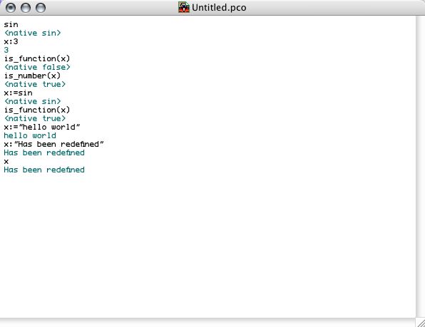
Notice that, at the end there are actually two versions of x. The former version is no longer accessible (in our example, but this can be different when variables are used from within different scopes). Here we simple mention this to stress the difference between variable definition and variable assignment. The former creates a new entry in the dictionary. The latter overrides an existing entry in the dictionary. If the variable does not exist, an assignment expression will fail.
Apart from defining variables, it is also possible to declare them. Declaring a variable is exactly the same thing, except for the fact that the name will be installed as constant instead of as an assignable variable. Declaration is done with a double colon instead of a single colon.
Notice that definitions and assignments are expressions. So they also have a value. This enables expressions like x:=(y::(x:4))+5 which will first define x to be 4, then declare the constant y to be the result thereof (i.e. 4) and subsequently assign the value of x to be 9. The result is that there are 2 variables: x associated with the value 9, and y associated with 4.
As already indicated by the above examples, functions (both natives and others) are called using ordinary calculus style: a function named f with arguments a1, a2 and a3 is called with an expected expression f(a1,a2,a3). Pico arguments are always evaluated one by one from left to right.
Functions are defined with the colon notation. E.g., the factorial function looks as follows:
fac(n):if(n=0,1,n*fac(n-1))
Notice that a function name can also be used just to refer the function, i.e. without calling it.
Functions "remember" the variables that existed when they were defined. Hence, functions keep a reference to the dictionary that was valid at the time of definition. It is said that Pico is lexically scoped. This also means that functions have "their own" variables. Variables (and functions) defined locally to functions are only visible to the code of those functions, and not outside those functions.
The following screen shot shows how functions are treated in Pico. It is worthwile studying the interaction as it shows some subtle interactions between the concepts introduced so far.
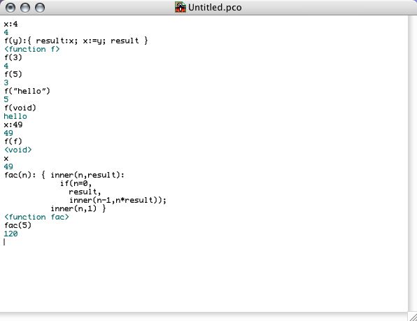
The function f uses the global variable x to store its previous argument. It uses a local variable result each time it is called. By (re)defining x in the global dictionary, f will use the old x and the old x is no longer accessible from within the main window. fac uses a local function inner that is only visible inside fac. inner also illustrates how functions with more than one argument are called.
Just like with variables, functions can also be declared instead of defined. The syntax is the same except for the colon which is replaced by a double colon. Since most programmers will not use the assignment operator for functions (however, there are some meaningful applications of this), it is more common to declare functions than to define them.
Notice that function bodies can be compound expressions, separated by semicolons and grouped together by curly braces. However, this is not essential to Pico. The curly braces are mere syntactic sugar for a call to the native begin function, i.e.
begin (e1, e2, ..., en) = {e1; e2; ...; en}
Since arguments of function calls (and hence also arguments of begin calls) are evaluated from left to right, begin does what it is expected to do.
Operators
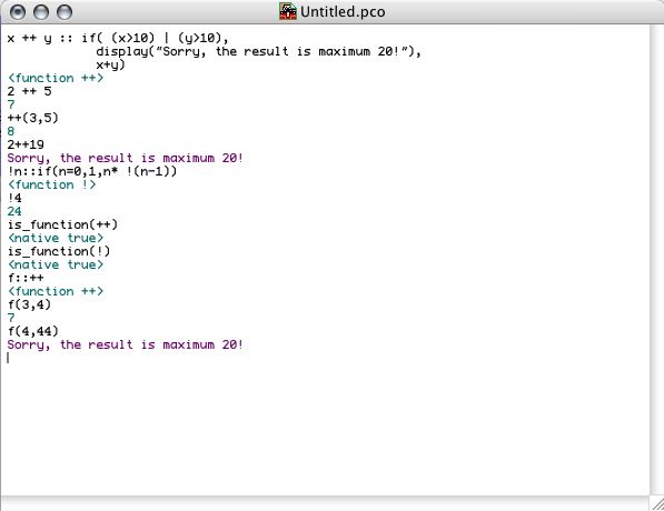
Functions with a special name consisting of only characters from the set {$, %, +, -, |, ~, &, *, \,/, !, ?, ^, #, <, =, >} are called operators. Although Pico internally treats operators in exactly the same way as other functions, their syntactic appearance is different. Pico operators (both unary - with 1 argument - and binary - with 2 arguments -) can be defined using familiar infix notation. But this is not compulsory. This is all shown by the following interaction:
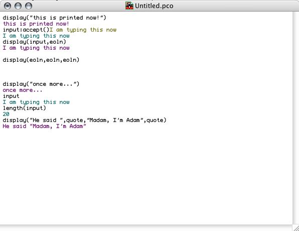
Two built-in functions are used for basic input-output in Pico:
A built-in variable eoln (actually a Pico text) can be used for generating line breaks. Also note that the result of accept is always a text. If one needs a number, one has to use a conversion function to convert the text to a number. Have a look at the interaction:
We have already seen the usage of some of Pico's native functions such as + and |. In fact as we will see below, "keywords" like if and while are also normal functions in Pico. The following table gives an overview and a brief explanation of the native functions in Pico:
| +, -, *, /, //, \\, ^ | arithmetic |
| <, <=, =, !=, x>y, x>=y | relational |
| ~, !~ | equivalence of references (e.g. tables) |
| trunc(x) | truncation |
| abs(x) | absolute value |
| char(n) | 1-character text corresponding to ASCII n |
| ord(t) | ASCII of 1-character text |
| number(t) | number or fraction value of text t |
| text(v) | textual representation of number or fraction v |
| random() | generates random number |
| clock() | seconds since startup |
| sqrt, sin, cos, tan, arcsin, arccos, arctan, exp, log | transcendental functions |
| length(t) | length of text t |
| explode(t) | explode text t into table of 1-character texts |
| implode(t) | pack table of 1-character texts as a text |
| is_void,is_number,... | type checking |
| size(t) | size of a table t |
| table@t | inline table creation |
| p#q | pairing (cons) in a table of size 2 |
| display@args | output |
| accept() | input |
| true, false, &, |, ! | boolean algebra |
| begin@lst | |
| if(b,cns(),alt()) | if construction |
| if(b,cns()) | if without alternative |
| while(pred(),exp()) | leading decision loop |
| until(pred(),exp()) | trailing decision loop |
| for(ini,pred(),inc(),exp()) | bounded loop |
| case@lst | jump-table driven case expecting tag/value pairs |
| load(txt) | load and evalute a file |
| dump(exp,text) | not yet implemented |
| read(txt) | parse a text as a pico expression |
| eval(exp) | evaluate an expression |
| print(exp) | pretty-print an expression |
| tag(exp) | get the tag identifying the expression tag |
| rank(exp) | return the number 'children' in exp's parse tree |
| make(nbr) | creates a parse tree node with tag nbr |
| get(exp,nbr) | read nbr'th child in the parse tree exp |
| set(exp,val,nbr) | change the nbr'th child in the parse tree |
| capture() | return current dictionary |
| commit(dct) | replace the current dictionary by dct |
| call(exp(continuation)) | call/cc |
| continue(cnt) | jump to the continuation |
| escape(exp()) | install a timed interupt |
| error@lst | generate an error dialog box |
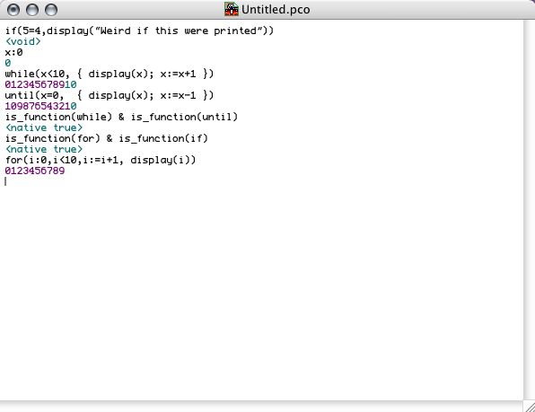
As we already explained, the "control flow keywords" like if and while are not really special Pico constructions but are mere primitive functions. This is also visible in the above table. As a matter of fact, these functions were actually implemented in Pico itself, but we will not go into the details of how this was done for now. The control flow functions if (2 variants), while (leading decision loop), until(trailing decision loop) and for (bounded loop) are illustrated in the following interaction. Notice that none of these functions create a new scope. This means that variables declared or defined in those functions are actually added to the dictionary in which the function is used.
Tables are Pico terminology for what is known as arrays or vectors in other programming languages. Tables are in principle one-dimensional and their indices range from 1 to the size of the table. If t is a table, then size(t) returns the size of the table.
Tables are defined or declared with an expression of the form t[index]:exp or t[index]::exp where index is an expression that should yield an number and t is a name under which the table will be installed in the dictionary. The special thing about Pico tables is that the exp will be evaluated repeately for every entry of the table. This allows for expressions like t[(i:0)+5]:(i:=i+1) in order to install an table of ascending numbers. When a table entry contains another table, the latter table can be accesses with the compound invocation t[i][j]. Pico allows this to be abreviated as t[i,j].
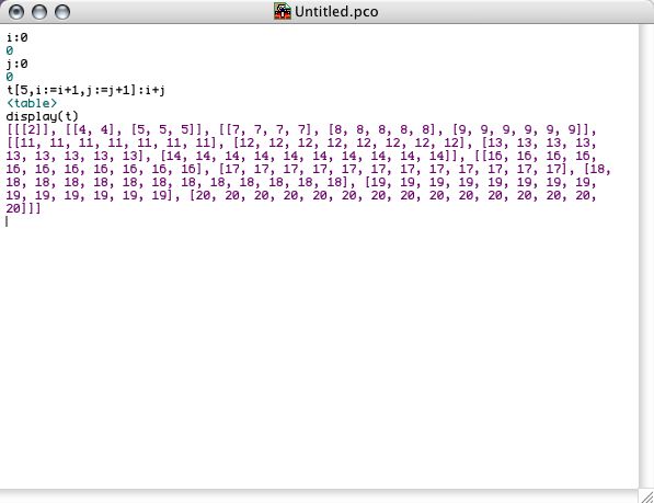
One special construction allows for a direct definition or declaration of multidimensional tables (which are internally stored as one dimensional tables whose entries are other tables). In order to illustrate this, we refer to the following screen shot. Notice that the size expression for higher dimensions is evaluated again and again. This allows, e.g., for the creation of upper triangular matrices in one line of code.
The table function is a native function that takes an arbitrary number of arguments (like begin) and returns those arguments packed in a table. Syntactic sugar is provided for this under the form of square brackets, in the same way curly braces are syntactic sugar for a call to begin. Hence:
table(e1, e2, ..., en) = [e1, e2, ..., en]
As explained before, begin and table are functions that take an arbitrary number of arguments. This is no exception. Pico functions that expect an arbitrary number of arguments can be defined using the @ notation:
f@args::body
This expression will install a function named f in the dictionary (of course: definition is also possible) that accepts a variable number of arguments. When called, the arguments are collected in a table which will be passed to the function under the name arg. Inside the body of the function, the table can be manipulated.
Now that we have shown this, we can reveal the true nature of begin and table:
begin@lst::lst[size(lst)]
table@lst::lst
Both accept any number of arguments (which will be evaluated from left to right). table merely returns the table of arguments. begin returns the last element of the table, i.e. the value of the last expression that was used in the call to begin.
The @ notation for functions is somewhat related to the @ operator. Apart from using @ as a notation for definition and declaration of variable length argument functions, @ is also used as an operator that consumes a function and an expression that evaluates to a table, and that applies the function to values in the table. This is exemplified in the following interaction:
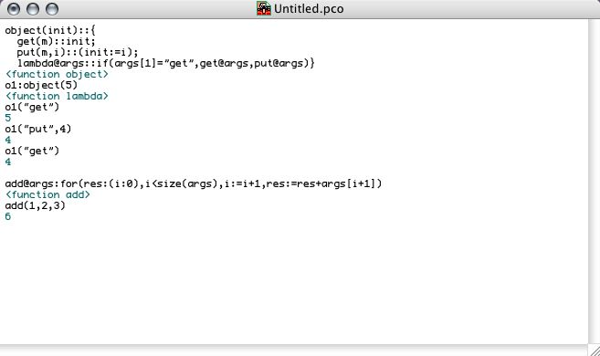
Study the examples carefully:
In Pico, functions can have two kinds of parameters: normal parameters and functional parameters. The precise kind of the parameter is syntactically visible. Binding actual arguments to formal parameters happens differently. In the case of normal parameters (i.e. the parameter is a normal name as in fac(n):if(n=0,1,n*fac(n-1)) ), the argument is evaluated and the associated value is bound to the formal parameter before the body of the function is evaluated.In order to describe the behaviour associated to functional parameters, it is best to look at an example:
zero(a, b, f(x), epsilon):{
   c: (a+b)/2;
   if(abs(f(c)) < epsilon,
      c,
      if(f(a)*f(c) < 0,
         zero(a, c, f(x), epsilon),
         zero(c, b, f(x), epsilon))) }
This Pico function looks for a zero of a function f(x) between a and b given a precision epsilon. The fact that f(x) is a functional argument results in the third expression (upon calling zero) never to be evaluated. When calling zero with 4 arguments, the first, the second and the fourth will be evaluated. But the third argument will be taken as an expression (depending on x) to be used as the body for a newly defined function called f of one parameter x. Hence, the way to call zero is zero(-1,1,x*2-5,0.001). The result is that inside zero, 4 names are accessible: a, b, f and epsilon. f happens to be bound to a function of one argument x (which is NOT visible inside zero) and body x*2-5.
This type of argument allows us to extend Pico in itself since functional parameters cause their arguments to be delayed. The following code excerpt shows how the Pico while function is programmed in Pico itself. In the same way, true, false, and, or and if where implemented as built-in functions that happen to delay some of their arguments:
while(cond(),body()): {
loop(value,pred):pred(loop(body(),cond()),value);
loop(void,cond()) }
The while function assumes the Church encoding of booleans:
true(t(),f()):t()
false(t(),f()):f()
These examples show how functional parameters (of zero arguments in these cases) allow for automatic thunk creation upon calling a function. This is in contrast to languages like SmallTalk or Self where one has to manually delay arguments by wrapping them in a function:
expression ifTrue: [ ... ] ifFalse: [ ... ]
In languages like Scheme it is the name of the "function" (like if) that determines what will happen.
A Pico expression is always evaluated with respect to an environment consisting of the variable bindings currently in the scope. In Pico nomenclature, this environment is called the dictionary. The dictionary can be conceived as a linked list associating names with values. Adding a new name to the dictionary always happens at the end of the linked list and looking up a name always starts at the end of the list and proceeds upward. Conceptually, the dictionary is a linked list of mutable and immutable names which result from definitions and declarations. Like anything in Pico, these dictionaries are first class and syntax and functions exist for manipulating them. The "current" dictionary is grabbed by calling the capture() native function with no arguments. The result is a dictionary that exposes a number of names. By definition, only the names that were declared (i.e. the immutable names) can be accessed from a dictionary. Trying to refer to a defined name will generate an error. This allows us to define modules or even simple objects in Pico. The following code excerpt shows how these dictionaries are used in conjunction with a qualified dot operator to access the declared names of a dictionary.
{ Stack()::{
    stk:void;
    psh(e)::
    stk:=[e,stk];
    pop() ::
      if(is_void(stk),
        error("pop from empty stack"),
        { e:stk[1];
          stk:=stk[2];
          e });
   capture() };
 s1::Stack();
 s1.psh(2);
 s1.pop()}
The example shows a "constructor" function Stack that defines a local variable stk and declares two functions. Then the "current" dictionary is grabbed by calling capture() and returned from the constructor function. The two dot qualification expressions show how the declared names can be used in the dictionary.
First class dictionaries can be seen as Pico's answer to objects and modularity.
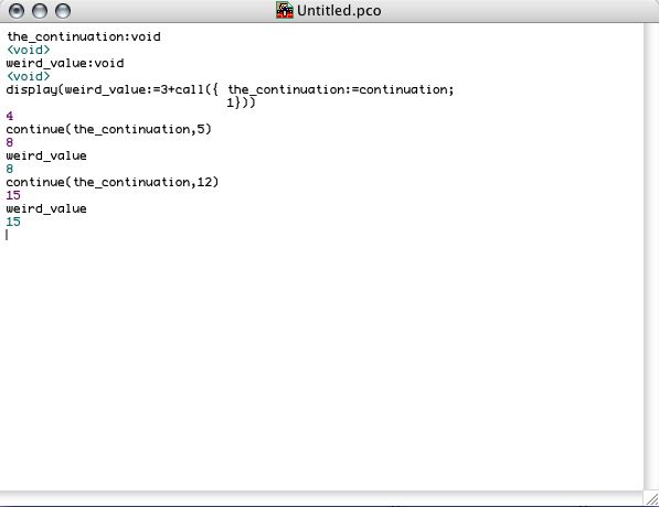
Pico features first class continuations. In contrast to Scheme's continuations, Pico's continuations are not aligned with functions, but are treated as a separate kind of value for which the is_continuation primitive exists. Two primitive functions call and continue can be used to grab the current continuation and to "jump" to a continuation. call is the same as call/cc in Scheme. In Pico, call takes an expression that depends on the parameter continuation. Hence, the formal heading of call is
call(exp(continuation)): ...
When provided with an expression, call will immediately evaluate that expression with continuation bound to the current continuation. That continuation can e.g. be stored in a variable and used later on in conjunction with continue. continue takes two arguments. The first has to be a continuation and the second has to be a value that will be returned at and substituted for the orignal call to call. The following interaction illustrates this.
Continuations are not easy to grasp at first and we will not explain them in detail in this small tutorial. We refer to the courseware of "Interpretation of Computer Programs II" where a lot of energy is spent on continuations. Part of that courseware is an introductory text on continuations.
A very representative usage of continuations is the implementation of an exception handling sytem which can be found in the Pico Extensions example in the sample code.
Pico programs are internally represented as a tree. This tree is accessible in Pico as a tagged table whose subtrees (also tables) can be gotten and set using the get and set primitives. Every tree is identified by a tag, which is a number. The Meta Abstractions file in the sample code exemplifies how these trees are manipulated.